EDock-ML (0.0.1-alpha) User Guide

 

Credits

Made by Tanay Chandak under the direction of Chung Wong.  Developed with the help of Armaan Chandak. John Mayginnes provided the docking data (used in the publication ¹) for training the machine-learning models.

 

Overview

EDock-ML allows a user to evaluate the likelihood of a compound to be active for a protein target by performing ensemble docking with the aid of machine learning.  The method is described in reference ¹.  The key idea is to dock a compound to an ensemble of structures rather than to a single structure, and employ machine learning to improve the use of docking scores to make predictions.  All dockings are performed by AutoDock Vina.²

EDock-ML automates the workflow for performing ensemble docking with machine learning.  A user supplies a compound by providing an ID from the ZINC database³ or by uploading a file.  The file can be in pdbqt format used by AutoDock Vina.² It can also be in mol2 format.  EDock-ML uses Open Babel ⁴ to convert mol2 to pdbqt files.   EDock-ML then provides data to help the user judge the likelihood of the compound to be active for a selected protein target.

This version provides four machine-learning models (k nearest neighbor, logistic regression, random forest, and support vector machine) for 24 protein kinases.  These models were already trained by using docking results from almost 400,000 compounds.  Users can use these models to obtain results quickly.   The major computational time will be spent on docking by AutoDock Vina.  If enough processors are available to perform docking to all the structures in parallel, the time to obtain results is determined by the docking to the structure taking the longest time.  This initial server provides only four processing cores.  We shall move to a server with more processors later.

Although we shall continue to add machine-learning models to EDock-ML, this version provides an option for users to train their own models if they have already performed docking on a large number of actives and decoys by AutoDock Vina.²

We also provide an option for users to perform docking only, if the users want to use the docking scores to an ensemble of structures in other ways.

EDock-ML provides three major menus for performing three major tasks: docking followed by prediction with machine learning, docking without using machine learning, using machine learning with user-provided docking scores to predict whether a compound is active.  These menus can be accessed from the bottom half of the home page, or from the pulldown menu accessible from the button labeled “Run Models” at the home page or “Run” at the top of the other pages.

 

Ensemble docking with machine learning for pre-trained proteins

To use this option, one selects the option “Docking + Machine Learning”.  In the web page that comes up, select “Use Stored Proteins”. 

Two buttons are available for selecting a ligand. “Choose File” allows a user to upload a file in pdbqt format used by AutoDock Vina.  If one enters a file in mol2 format, it will be converted by Open Babel into the pdbqt format.  “Retrieve from Zinc” allows a user to enter an ID from the ZINC database.³

Once the ligand has been validated, one can hit the box with “Select Protein” displayed to select one of the proteins with machine-learning models already trained.  When the button “Begin Docking” becomes active, click it to begin docking. At this point, you will be redirected to the results page, where you will see the jobs running or the queue positions of your docking processes. Furthermore, in the results page, you will get access to the ‘external link.’ Upon saving and reentering this link at a later time, you will still see the same data displayed in the results tab.

 

After the docking is done, a user is presented with the buttons “Run All Models”. Clicking this button will run all the four machine-learning models to estimate the likelihood of the compound to be active.  The results are presented in a table like this:

 

 

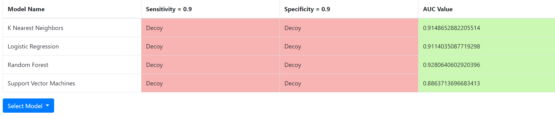
It gives the Area Under Receiver Operating Characteristic Curve (AUC) for each machine-learning model on the far right so that a user can get an idea on how well each model classifies compounds into actives and inactives for the protein selected.  Each value varies between 0 and 1 with 1 giving the best possible model.  A value of 0.5 means that the model performs only as well as a random model does.  It also predicts whether the compound is active or inactive (decoy) for a model giving a specificity of 0.9, and a model giving a sensitivity of 0.9.  If every model in the column labeled “Specificity = 0.9” predicts the compound to be active, the machine-learning models predict that the compound would be active with better than 90% probability.  If no model under the column labelled “sensitivity = 0.9” predicts active, the machine-learning models predict 90% chance that the compound is inactive.  However, results are not always that clear cut.  For example, two models may predict the compound to be active under the column labelled “Specificity = 0.9” but the other two may not.  The AUCs give you some ideas which models you may want to believe more.  Besides the AUCs, EDock-ML also displays the Receiver Operating Characteristic Curves (ROCs) to help you make decision.  Here is an example of a ROC:

 

 

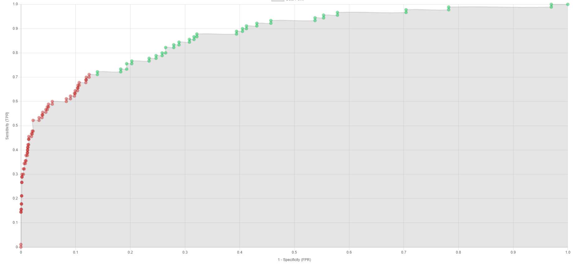
From this curve, you may see that models choosing a specificity ~ 0.86 (1- specificity = 0.14) or smaller would have predicted the compound to be active (points colored green).  0.86 still gives a small false positive rate, although slightly less well than 0.9.  In this case, the odds that your compound is active is still high, especially if other machine-learning models also predict this compound to be active at high specificity.

 

You may also click on each point on the graph to show more details:

 

 

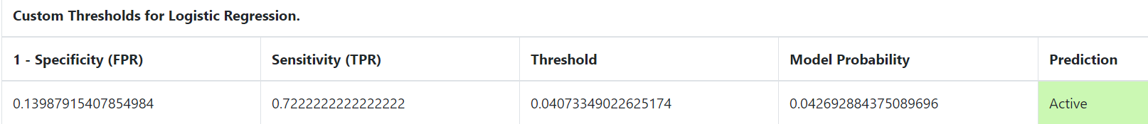
It gives the specificity and the sensitivity of the point chosen.  It also displays the probability calculated from the selected machine-learning model for your compound and the threshold used to divide actives and decoys for that point.

 

The button “Select Model” allows one to select the ROC of another machine learning model to examine.

 

The button “Save Data to Image” allows one to save the results to a pdf file.

 

 

Ensemble docking with machine learning via user-supplied training data

 

If you have already performed molecular docking studies on a large number of actives and decoys for a protein, you may use them to train your own machine-learning models, and predict whether other compounds are likely to be active.

 

To do this, instead of choosing the button “Use Stored Proteins”, you choose “Upload Custom Structures”.  You may then select a ligand by using the button “Choose File” or “Retrieve from Zinc” as described above.  Here, you have to upload your own pdbqt and config files for the protein of interest.  These files need to be prepared according to the specifications of AutoDock Vina.²  You may upload the files for each structure one at a time by using the button “Upload One at a Time” or select all the files for all the structures at once by selecting the option “Select Multiple”.  Once a window opens up, you may highlight the files you would like to upload to EDock-ML.

 

Once the button “Begin Docking” becomes active, click it to start docking the ligand to the ensemble of structures that you have uploaded. Once the docking has been completed, you will see a table that looks like this:

 

 

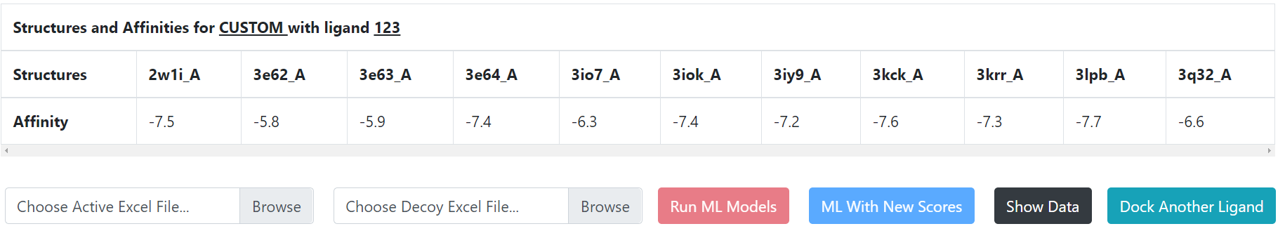
It contains the docking scores of your compound to each structure.  You now also see two fields for uploading Excel files containing the docking scores of actives and decoys that can be used to train the four machine-learning models. The field with “Choose Active Excel File” displaced allows you to upload an Excel file containing the docking scores of known actives.  The field with “Choose Decoy Excel File” displaced allows you to upload an Excel file containing the docking scores of inactive compounds.  The top row of each Excel file contains the IDs labeling your protein structures.  Each other row contains the docking scores of a compound to the protein structures.  You may then click “Run ML Models” to start training the machine-learning models and predict whether the compound you entered at the beginning is likely to be active.

 

On this page, you may also see another button “Dock Another Ligand”.  This allows you to repeat the above process for another ligand.  By repeating this process, you may study more compounds.  Note that the machine-learning models are only trained for the first ligand. EDock-ML saves them so that they do not need to be re-trained when studying the second and later ligands.

 

Docking menu

You may perform docking without machine learning under the “Docking” menu.  Again, you may dock compounds to the proteins already stored in the database of EDock-ML, or to a protein that you provide.

 

Docking using stored proteins

This follows the procedure described in the section on docking + machine learning except that the option for performing machine learning is not shown until the docking is done.  If your goal is just to obtain docking scores to the ensemble of structures of a stored protein, you may record your docking scores after the docking runs have been completed and do not continue with machine learning.   However, if you would like to perform machine learning as well, you may click the button “Show ML Options” that makes the option “Run All Models” available. Clicking this button will run the machine-learning models as described above on docking with machine learning.

 

Docking to your own proteins

If you have prepared the pdbqt and configuration files for a protein that you are interested in studying, you may upload them to EDock-ML so that you may dock different ligands to them.  To use this option, you click the button “Upload Custom Structures”. After supplying a ligand via “Choose File” or “Retrieve from Zinc”, you may upload your pdbqt and configuration files for your protein in two different ways.  To enter these files for one protein structure at a time, use the button “Upload One at a Time”.  The fields showing “Choose Configuration File” and “Choose PDBQT File” allow you to upload these files.  You may use the button “Add Another Structure” to add more structures.  Once all structures have been added, you may start docking when the button “Begin Docking” becomes active.  You may also upload all the configuration and pdbqt files in one go by choosing “Select Multiple”.  Once a window has opened up, browse to the folder containing your files and highlight the files to be uploaded.

 

Once docking is done, you are offered the options “Show ML Options” or “Dock Another Ligand”.  The former allows you to train machine-learning models as described above for docking + machine learning using custom structures, and use the models to predict whether your compound is active.

 

The button “Dock Another Ligand” allows you to dock more ligands to the protein of interest.

 

Machine Learning

 

Again, two options are available.  You may use the stored proteins with machine-learning models already trained to predict whether your compound is active if you already have its docking scores obtained outside of EDock-ML.  For proteins not yet developed and stored in EDock-ML, you may provide your own data to train machine-learning models and use them for predictions.

 

For using a stored protein, select “Machine Learning” and then “Use Stored Proteins” in the page that comes up. 

 

You may experiment with the machine-learning models by using docking scores of some sample actives or inactives.  To do this, click “Select Proteins” to choose a protein, click “Choose Test #” to select a test set, click “Use Sample Active Scores” to use the docking scores of the active compound in the set, or click “Use Sample Decoy Scores” to use the docking scores for the inactive compound in the set.

 

If you have already docked your compound with the AutoDock Vina before using EDock-ML, you may enter the docking scores into EDock-ML to predict whether your compound is active.  To begin, click “Find Structures” to open up a menu for entering your docking scores.  You may enter the docking scores as a JSON object by selecting “Use JSON Text Box”.  However, many users may find “Use Smaller Text Boxes” easier to use.  The small boxes allow you to enter the docking scores for the structures which IDs are displayed.  After all the numbers have been entered, the button “Run All Models” becomes active.  (If not, click once outside the button/text-boxes.) Click it to use the pre-trained machine-learning models to predict the likelihood of your compound to be active.

 

If you have already performed docking with AutoDock Vina for a large number of actives and decoys, you may upload the data to EDock-ML to train the machine-learning models yourself and use them to predict whether a supplied compound is likely to be active.

 

For this, you would click “Upload Custom Structure”.  A box opens up to allow you to browse your disk to upload an Excel File containing the docking scores of compounds to an ensemble of structures.  This may be one of the two Excel files described below.  It is used to create a form for you to enter the docking scores of a compound that you would like to predict whether it is active.  The form will be available after you have clicked “Create Form”.  After entering the scores, click “continue” to open up the menu:

 

 

This allows you to upload two Excel files containing the docking scores for actives and inactives that can be used to train machine-learning models, by clicking “Run ML Models”.

 

If you would like to evaluate another compound, click “ML With New Scores” to enter the docking scores for this compound.  Predictions will come back quicker this time because the machine-learning models have already been trained after the first ligand.

 

 

References

 

1.         Chandak T, Mayginnes JP, Mayes H, Wong CF. Using machine learning to improve ensemble docking for drug discovery. Proteins: Structure, Function and Bioinformatics. 2020.

2.         Trott O, Olson AJ. Software news and update AutoDock Vina: Improving the speed and accuracy of docking with a new scoring function, efficient optimization, and multithreading. J Comput Chem. 2010;31(2):455-461.

3.         Sterling T, Irwin JJ. ZINC 15 - Ligand Discovery for Everyone. J Chem Inf Model. 2015;55(11):2324-2337.

4.         O'Boyle NM, Banck M, James CA, Morley C, Vandermeersch T, Hutchison GR. Open Babel: An open chemical toolbox. J Cheminf. 2011;3:33.